Isogeometric Analysis in MOOSE
This example illustrates using Isogeometric Analysis (IGA) within MOOSE framework to perform a simulation. This example simulates loads applied to a "c-frame" to determine the maximum principal stress.
Creating IGA Mesh
To create the mesh file included in this example a Coreform Cubit license is needed. Coreform Cubit is a product released and maintained by Coreform, LLC. A free to use Cubit Learn license can be acquired.
The following is not required to run the example, but is required to generate the input mesh that is included in the example. To execute the Cubit journal file in batch from the command line use the following command:
coreform_cubit -batch cframe_build.jou
Within the journal file, see Listing 1, there are unique commands that will generate a uspline on the discretized mesh.
Line 35 sets the degree and continuity of the uspline
As of this writing, the max degree supported by libmesh is 2.
All continuity must equal p-1 where p is the degree.
Line 36 constructs the uspline using the geometry as a basis.
Line 37 fits the uspline that was built to the geometry.
Listing 1: Complete Coreform Cubit file for generating IGA input mesh
import step "c-frame.step" heal
remove surface 15 17 21 19 22 23 16 25 18 20 24 26 14 35 38 33 34 36 37 7 8 4 5 6 1 2 10 12 3 9 13 11 80 77 81 88 79 86 90 78 76 89 87 75 91 85 29 28 30 27 31 32 62 60 57 58 48 45 47 50 49 46 54 53 51 56 52 55 41 39 42 43 40 44 68 66  extend
remove surface 93  extend
remove surface 94  extend
webcut volume 1  with sheet extended from surface 99 98 96  preview
webcut volume 1  with sheet extended from surface 99 98 96
webcut volume all with sheet extended from surface 92 59
webcut volume 6 4 3 5 1 2  with sheet extended from surface 67 61
webcut volume 1 16 2 15  with plane vertex 52  vertex 215  vertex 10  preview
webcut volume 1 16 2 15  with plane vertex 52  vertex 215  vertex 10
create vertex on curve 14  fraction 0.5 from start
create vertex on curve 77  fraction 0.5 from start
create vertex on curve 32  fraction 0.5 from start
webcut volume 16 2 15  with plane vertex 270  vertex 269  vertex 271
webcut volume 1  with plane vertex 270  vertex 269  vertex 271  preview
webcut volume 1  with plane vertex 270  vertex 269  vertex 271
delete Vertex 271 269 270
imprint all
merge all
volume all redistribute nodes off
volume all scheme Sweep Vector 1 0 0
volume all scheme Sweep Vector 1 0 0 sweep transform least squares
volume all autosmooth target on  fixed imprints off  smart smooth off
volume all size 0.5
mesh volume all
block 1 vol all
sideset 2 surf 194 203 196
sideset 3 Surface 146 155 148
block 1 element type hex27 #Quadratic FEA elements
export mesh "CFrame_FEA_05_deg2.e"  overwrite #FEA Export
set uspline vol all deg 2 cont 1
build uspline vol all as 1
fit uspline 1
export uspline 1 exodus "CFrame_IGA_05"
MOOSE-IGA Simulation
Performing the simulation utilizing the mesh created above does not require much with respect to the MOOSE input, simply load the mesh from a file and select utilize the RATIONAL_BERNSTEIN element family as shown in Listing 2. Exporting using the VTK format (vtk = true) input will output in a format that will capture the higher-order nature of the IGA based elements using Paraview visualization.
Listing 2: Complete input file for running example problem with IGA in MOOSE.
[GlobalParams]
  displacements = 'disp_x disp_y disp_z'
[]

[Mesh]
  [igafile]
    type = FileMeshGenerator
    file = cframe_iga_coarse.e
    clear_spline_nodes = true
  []
[]

[Variables]
  [disp_x]
    order = SECOND
    family = RATIONAL_BERNSTEIN
  []
  [disp_y]
    order = SECOND
    family = RATIONAL_BERNSTEIN
  []
  [disp_z]
    order = SECOND
    family = RATIONAL_BERNSTEIN
  []
[]

[Kernels]
  [TensorMechanics]
#Stress divergence kernels
    displacements = 'disp_x disp_y disp_z'
   []
[]

[AuxVariables]
    [von_mises]
        #Dependent variable used to visualize the von Mises stress
       order = SECOND
       family = MONOMIAL
    []
    [Max_Princ]
       #Dependent variable used to visualize the Hoop stress
       order = SECOND
       family = MONOMIAL
    []
    [stress_xx]
        order = SECOND
        family = MONOMIAL
    []
    [stress_yy]
        order = SECOND
        family = MONOMIAL
    []
    [stress_zz]
        order = SECOND
        family = MONOMIAL
    []
[]

[AuxKernels]
  [von_mises_kernel]
    #Calculates the von mises stress and assigns it to von_mises
    type = RankTwoScalarAux
    variable = von_mises
    rank_two_tensor = stress
    scalar_type = VonMisesStress
  []
  [MaxPrin]
    type = RankTwoScalarAux
    variable = Max_Princ
    rank_two_tensor = stress
    scalar_type = MaxPrincipal
  []
  [stress_xx]
    type = RankTwoAux
    index_i = 0
    index_j = 0
    rank_two_tensor = stress
    variable = stress_xx
  []
    [stress_yy]
    type = RankTwoAux
    index_i = 1
    index_j = 1
    rank_two_tensor = stress
    variable = stress_yy
  []
  [stress_zz]
    type = RankTwoAux
    index_i = 2
    index_j = 2
    rank_two_tensor = stress
    variable = stress_zz
  []
[]

[BCs]
  [Pressure]
    [load]
      #Applies the pressure
      boundary = '3'
      factor = 2000 # psi
    []
  []
  [anchor_x]
    #Anchors the bottom and sides against deformation in the x-direction
    type = DirichletBC
    variable = disp_x
    boundary = '2'
    value = 0.0
  []
  [anchor_y]
    #Anchors the bottom and sides against deformation in the y-direction
    type = DirichletBC
    variable = disp_y
    boundary = '2'
    value = 0.0
  []
  [anchor_z]
    #Anchors the bottom and sides against deformation in the z-direction
    type = DirichletBC
    variable = disp_z
    boundary = '2'
    value = 0.0
  []
[]

[Materials]
  [elasticity_tensor_AL]
    #Creates the elasticity tensor using concrete parameters
    youngs_modulus = 24e6 #psi
    poissons_ratio = 0.33
    type = ComputeIsotropicElasticityTensor
  []
  [strain]
    #Computes the strain, assuming small strains
    type = ComputeSmallStrain
    displacements = 'disp_x disp_y disp_z'
  []
  [stress]
    #Computes the stress, using linear elasticity
    type = ComputeLinearElasticStress
  []
  [density_AL]
    #Defines the density of steel
    type = GenericConstantMaterial
    prop_names = density
    prop_values = 6.99e-4 # lbm/in^3
  []
[]

[Preconditioning]
  [SMP]
    #Creates the entire Jacobian, for the Newton solve
    type = SMP
    full = true
  []
[]

[Postprocessors]
  [max_principal_stress]
    type = PointValue
    point = '0.000000 -1.500000 -4.3'
    variable = Max_Princ
    use_displaced_mesh = false
  []
  [maxPrincStress]
    type = ElementExtremeValue
    variable = Max_Princ
  []
[]

[Executioner]
  # We solve a steady state problem using Newton's iteration
  type = Steady
  solve_type = NEWTON
  nl_rel_tol = 1e-9
  l_max_its = 300
  l_tol = 1e-4
  nl_max_its = 30
  petsc_options_iname = '-pc_type -pc_hypre_type -ksp_gmres_restart'
  petsc_options_value = 'hypre boomeramg 31'
[]

[Outputs]
  vtk = true
[]
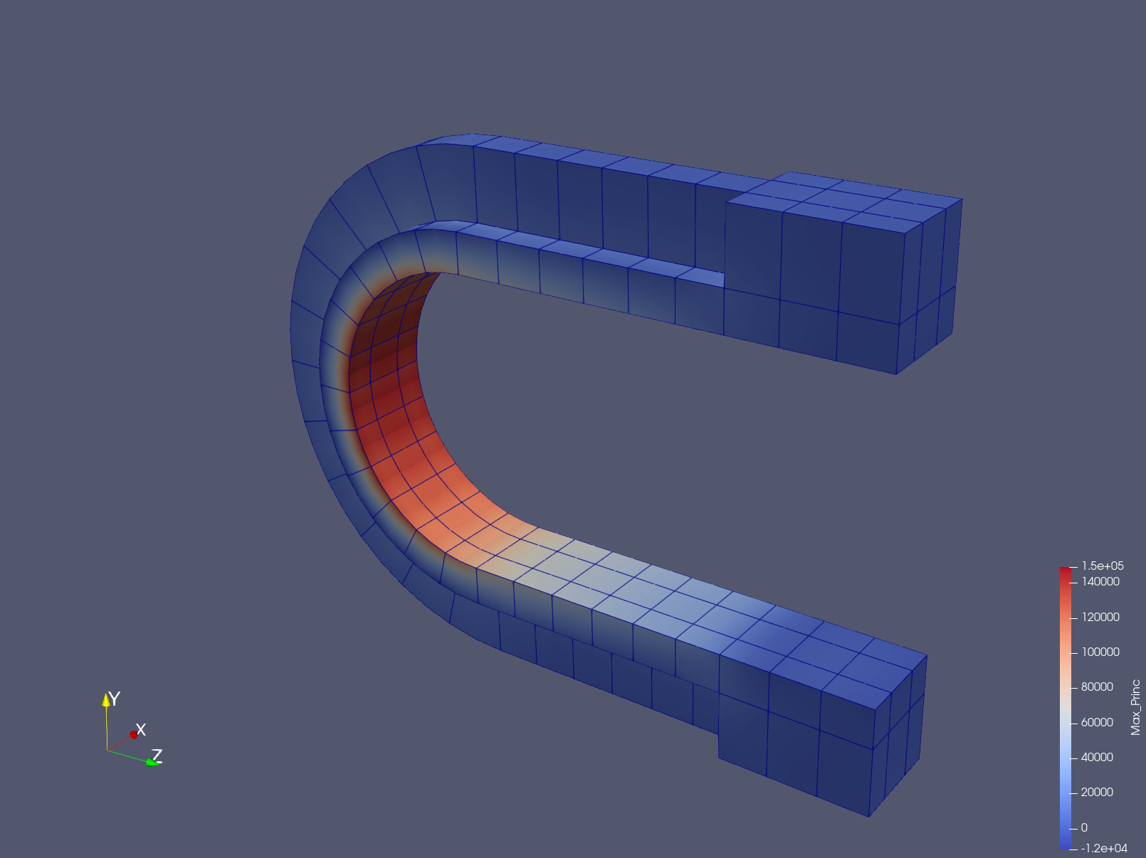
Figure 1: Maximum principal stress for "c-frame" example utilizing IGA in MOOSE.